Overview
Teaching: 10 min Exercises: 5 minQuestions
Can we calculate things in parallel?
Objectives
Use Dask to parallelize Python computations
Use Dask arrays to analyze data that naturally comes in arrays
Dask takes yet another approach to speeding up Python computations. One of the main limitations of Python is that in most cases, a single Python interpreter can only access a single thread of computation at a time . This is because of the so-called Global Interpreter Lock (or GIL).
And while there is a multiprocessing module in the Python standard library, it’s use is cumbersome and often requires complicated decisions. Dask simplifies this substantially, by making the code simpler, and by making these decisions for you.
Dask delayed computation:
Let’s look at a simple example:
The following are some very fast and simple calculations, and we add some
sleep into them, to simulate a compute-intensive task that takes some
time to complete:
import time

def inc(x):
    time.sleep(1)
    return x + 1

def add(x, y):
    time.sleep(1)
    return x + y
Consider the following calculation:
x1 = inc(1)
x2 = inc(2)
z = add(x1, x2)
How long would it take to execute this?
Notice that while z depends on both x1 and x2, there is no
dependency between x1 and x2. In principle, we could compute both of
them in parallel, but Python doesn’t do that out of the box.
One way to convince Python to parallelize these is by telling Dask in advance about the dependencies between different variables, and letting it infer how to distribute the computations across threads:
from dask import delayed

x1 = delayed(inc)(1)
x2 = delayed(inc)(2)
z = delayed(add)(x1, x2)
Using the delayed function (a decorator!) tells Python not to perform
the computation until we’re done setting up all the data dependencies.
Once we’re ready to go we can compute one or more of the variables:
z.compute()
How much time did this take? Why?
Dask computes a task graph for this computation:
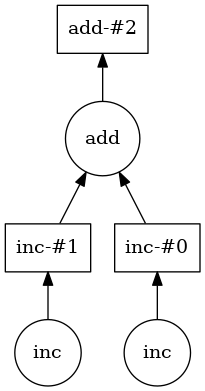
Once this graph is computed, Dask can see that the two variables do not depend on each other, and they can be executed in parallel. So, a computation that would take 2 seconds serially is immediately sped up n-fold (with n being the number of independent variables, here 2).
Let’s do something slightly more interesting (and neuro-related):
Let’s say that we’d like to compute the tsnr over several runs of fMRI data, for example, using the open-fMRI dataset ds000114:
from glob import glob

fnames = glob('/data/ds000114/sub-01/ses-test/func/*.nii.gz')
This is a list with 5 different file-names, for the different runs during this session.
One way to calculate the tsnr across is to loop over the files, read in the data for each one of them, concatenate the data and then compute the tsnr from the concatenated series:
import nibabel as nib #in case it is not loaded and to prevent the confusing error
data = []
for fname in fnames:
    data.append(nib.load(fname).get_data())

data = np.concatenate(data, -1)
tsnr = data.mean(-1) / data.std(-1)
Lazy loading in Nibabel
Nibabel uses “lazy loading”. That means that data are not read from file until when the nibabel
loadfunction is called on a file-name. Instead, Nibabel waits until we ask for the data, using theget_datamethod of TheNifti1Imageclass to read the data from file.
When we do that, most of the time is spent on reading the data from file. As you can probably reason yourself, the individual items in the data list have no dependency on each other, so they could be calculated in parallel.
Because of nibabel’s lazy-loading, we can instruct it to wait with the
call to get_data. We create a delayed function that we call
delayed_get_data:
delayed_get_data = delayed(nib.Nifti1Image.get_data)
Then, we use this function to create a list of items and delay each one of the computations on this list:
data = []
for fname in fnames:
    data.append(delayed_get_data(nib.load(fname)))

data = delayed(np.concatenate)(data, -1)
tsnr = delayed(data.mean)(-1) / delayed(data.std)(-1)
Dask figures that out for you as well:
tsnr.visualize()
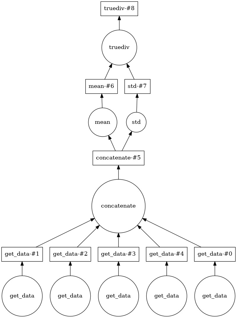
And indeed computing tsnr this way can give you an approximately 4-fold speedup. This is because Dask allows the Python process to read several of the files in parallel, and that is the performance bottle-neck here.
Dask arrays
This is already quite useful, but wouldn’t you rather just tell dask that you are going to create some data and to treat it all as delayed until you are ready to compute the tsnr?
This idea is implemented in the dask array interface. The idea here is that you create something that provides all of the interfaces of a numpy array, but all the computations are treated as delayed.
This is what it would look like for the tsnr example. Instead of
appending delayed calls to get_data into the array, we create a series
of dask arrays, with delayed_get_data. We do need to know both the shape
and data type of the arrays that will eventually be read, but
import dask.array as da

delayed_arrays = []
for fname in fnames:
    img = nib.load(fname)
    delayed_arrays.append(da.from_delayed(delayed_get_data(img),
                          img.shape,
                          img.get_data_dtype()))
If we examine these variables, we’ll see something like this:
[dask.array<from-value, shape=(64, 64, 30, 184), dtype=int16, chunksize=(64, 64, 30, 184)>,
 dask.array<from-value, shape=(64, 64, 30, 238), dtype=int16, chunksize=(64, 64, 30, 238)>,
 dask.array<from-value, shape=(64, 64, 30, 76), dtype=int16, chunksize=(64, 64, 30, 76)>,
 dask.array<from-value, shape=(64, 64, 30, 173), dtype=int16, chunksize=(64, 64, 30, 173)>,
 dask.array<from-value, shape=(64, 64, 30, 88), dtype=int16, chunksize=(64, 64, 30, 88)>]
These are notional arrays, that have not been materialized yet. The data has not been read from memory yet, although dask already knows where it would put them when they should be read.
We can use the dask.array.concatenate function:
arr = da.concatenate(delayed_arrays, -1)
And we can then use methods of the dask.array object to complete the
computation:
tsnr = arr.mean(-1) / arr.std(-1)
This looks exactly like the code we used for the numpy array!
Given more insight into what you want to do, dask is able to construct an even more sophisticated task graph:
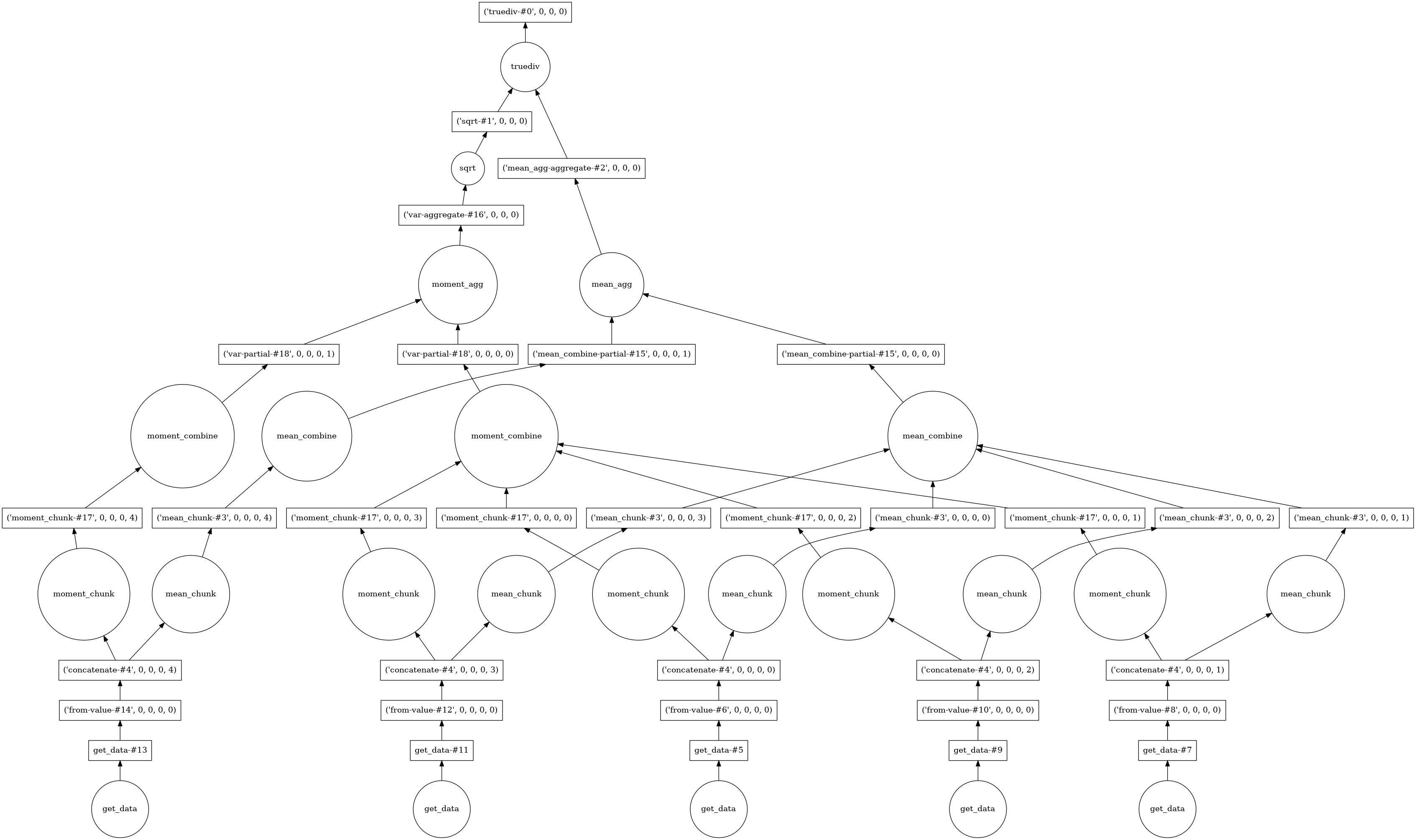
This looks really complicated, but notice that because dask has even more insight into what we are trying to do, it can delay some things until after aggregation. For example, the square root computation of the standard deviation can be done once at the end, instead of on each array separately.
And this leads to an approximately additional 2-fold speedup.
One of the main things to notice about the dask array is that because the data is not read into memory it can represent very large datasets, and schedule operations over these large datasets in a manner that makes the code seem as though all the data is in memory.
Key Points
If computations lend themselves to parallelization, they can be sped up substantially
Dask arrays can speed up things even more, for array data
Dask provides a whole universe of tools for parallelization