Overview
Teaching: 15 min Exercises: 0 minQuestions
Why use artifical neural networks?
What is the mechanism of learning in neural networks?
Objectives
Understand the history of neural networks
Write code to mimic very small networks
Implement back-propagation for very small networks
Why neural networks? Why now?
Artifical neural networks are not a new idea at all. Arguably, these ideas were around at the dawn of computer science, in the 1940’s, and were clearly articulated in work that continued in the 1950’s and 1960’s. In the 1980’s this thinking was put to practice in the work of several groups including the PDP (parallel distributed programming) research group. But it was really only in the 1990’s that computers could be programmed to do highly useful things with neural networks. For example, the seminal work of Yann LeCun developing convolutional neural networks that were able to read hand-written digits.
However, the implementation and application of neural networks to many different problems really took off in the early 2010’s with work that spanned academic and industry research labs (e.g., work from Andrew Ng’s group at Stanford, in collaboration with researchers at Google, as well as work from Geoff Hinton’s group and Yoshua Bengio, both at the time in Canada, Toronto and Montreal, respectively).
Some of the factors that ushered in the current golden age of artificial neural networks are:
- Development of hardware and software to implement large neural networks. An important part of this is work that made computing some of the fundamental operations in neural networks very fast on graphical processing units (GPUs).
- The availability of large datasets for training these algorithms
- Theoretical developments across a wide range of fields, including ideas closely related to the structure of these networks, but also in cognate fields, such as optimization.
One of the landmark datasets that allow us to track these developments results for the field was the ImageNet dataset that includes millions of images from 1,000 different classes. This dataset is used as a benchmark for the performance of object classification systems. In 2012, a neural network algorithm was able to finally edge out other methods in terms of accuracy, and more recently these algorithms have reached parity with human performance.
Since that time, neural network algorithms have been used for a (increasingly large) number of other applications, including in the analysis of neuroimaging data.
How does a neural network work?
The simplest form of a neural network is essentially a regression problem:
Indulge me as I go through the mechanics and notation of this simple network
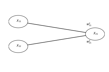
Variables indicated with are nodes and they can have levels of activity as real (or floating point) numbers. The first sub-script () indicates the layer to which this unit belongs and the second sub-script () indicates the (arbitrary) identity within the layer.
Weights between layers are indicated by . Here, we’ll use the super-script to indicate the target layer of the weight. First sub-script indicates the identity of the source unit and second super-script indicates the identity of the target unit.
So, this network would be implemented as (for example):
x11 = 1
x12 = 2
w_2_11 = -2
w_2_21 = 3

x21 = w_2_11 * x11 + w_2_21 * x12
Or alternatively:
x21 = np.dot([w_2_11, w_2_21], [x11, x12])
Here is a slightly more complicated network:
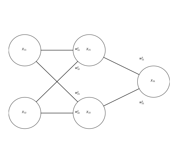
And its implementation in code:
x11 = 1
x12 = 2

w_2_11 = -2
w_2_21 = 3
w_2_12 = 2
w_2_22 = -3

w_3_11 = 3
w_3_21 = 2
To calculate the output of this one, we need to run several intermediate computations:
x21 = np.dot([w_2_11, w_2_21], [x11, x12])
x22 = np.dot([w_2_21, w_2_22], [x11, x12])

x31 = np.dot([w_3_11, w_3_21], [x21, x22])
Things get more interesting if we allow each unit to be non-linear, by applying some function to its input:

One popular function (inspired by the fI curve of neurons!) is a hyperbolic tangent:
x = np.arange(-np.pi, np.pi, 0.001)
plt.plot(x, np.tanh(x))

Another function that is similar in shape, but much simpler in other respects is the rectified linear unit:
def relu(x):
 return np.max([x, np.zeros(x.shape[0])], axis=0)

plt.plot(x, relu(x))

Our neural network then becomes:
x21 = relu(np.dot([w_2_11, w_2_21], [x11, x12]))
x22 = relu(np.dot([w_2_21, w_2_22], [x11, x12]))

x31 = relu(np.dot([w_3_11, w_3_21], [x21, x22]))
Training the network
Networks are trained through gradient descent: gradual changes to the values of the weights
The gradients are calculate through backpropagation: Error is propagated back through the network to calculate a gradient (derivative) for each weight by multiplying:
- The gradient of the loss function with respect to the node a weight feeds into
- The value of the node feeding into the weight
- The slope of the activation function of the node it feeds into
For example, for the network we had above, let’s assume the desired output was 10, instead of 12
# We take the simplest possible error, the absolute difference:
e31 = x31 - 10

# We'll use this helper function to derive ReLU functions:
def d_relu(x):
    if x > 0:
        return 1
    else:
        return 0

e_3_11 = e31 * x21 * d_relu(x31)
e_3_21 = e31 * x22 * d_relu(x31)

e_2_11 = e_3_11 * x11 * d_relu(x21)
e_2_21 = e_3_11 * x12 * d_relu(x21)

e_2_12 = e_3_21 * x11 * d_relu(x22)
e_2_22 = e_3_21 * x12 * d_relu(x22)
We set a small learning rate, that will determine how fast we move in the direction of the gradient:
lr = 0.01
And apply the change:
w_3_11 = w_3_11 - e_3_11 * lr
w_3_21 = w_3_11 - e_3_21 * lr

w_2_11 = w_2_11 - e_2_11 * lr
w_2_12 = w_2_12 - e_2_12 * lr

w_2_21 = w_2_21 - e_2_21 * lr
w_2_22 = w_2_22 - e_2_22 * lr
We calculate the resulting activations again:
x21 = relu(np.dot([w_2_11, w_2_21], [x11, x12]))
x22 = relu(np.dot([w_2_21, w_2_22], [x11, x12]))

x31 = relu(np.dot([w_3_11, w_3_21], [x21, x22]))
And repeat this process again and again, until convergence. If we had more than one observation for which we knew the input output relationship, we would use multiple samples to train the network, using each one one of these pairs.
A full run over all of the data is called an “epoch” of learning. Using some rather straightforward algebra, the same procedue can be used to learn from multiple samples at the same time. We call that a “batch”. In our case, the entire dataset is just one observation, so the epoch and batch both have size of one.
Key Points
Neural networks have been around for a while.
They’ve more recently become very useful.
The main learning mechanism in neural networks is back-propagation and gradient descent.